Here is a really cool transportation idea - using gravity powered vacuum tubes to travel through the earth across long distances - and all of that in 42 minutes. You can see the relevant part of a discovery channel show on this topic in the following youtube snippet.
Of course, there are many problems : continental drift, rotation of the earth's inner layers w.r.t. the surface and the incredible pressure and temperature closer to the center of the earth that make this project completely infeasible.
Irrespective of the hurdles, its still extremely interesting. Of all the coolness associated with this idea, the thing that really bakes ones noodle is the claim that any straight line journey through the earth takes 42 minutes. You don't need to be a Hitch Hiker's fan to be super excited by this. Additionally, the oldest records of this method of travel show that it was first proposed by Robert Hooke, for whom I have a soft spot in my heart (after reading The Scientists).
If you have read my other similarly themed blog post, you might already know that I love such things, and this was another opportunity to spend some time playing with physics, maths and programming. So I set out to find a closed form expression for the travel time across the earth and also verify the startling 42 minutes result.
We will start from the first principles and derive the travel time. To make it possible to solve this problem analytically, we will assume that the density of the earth (\(d_e\)) is uniform (which it is not and we will come to that bit later).
Lets imagine that we want to travel from point A to point B on the surface of the earth and we plan to do so via a straight line path through the bulk of the earth. Let the length of this path be d and let the minimum distance of this path from the center of the earth be p. Here is a diagram which makes this easier to imagine...
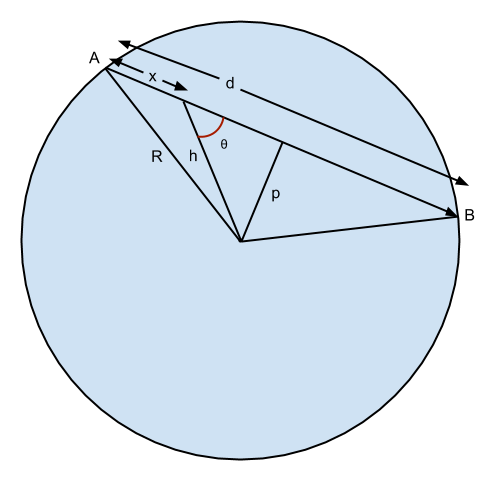
To describe the remaining quantities in the diagram,
- d : straight line distance between A and B.
- p : minimum distance of the straight line path from center of earth.
- R : radius of the earth (\(6.371\times10^6\) m)
- x : distance traveled by the train at time \(t_x\).
- h : distance of the train from the center of the earth at time \(t_x\).
- \(\theta\) : angle that the path at \(t_x\) makes with the force of gravity.
We will first find the time that the train takes to travel half of its path, and by symmetry, we know that the time of the other half is identical. This way, we won't have to muck around with the opposite acceleration (retardation) in the second half of the journey.
We know from Newton's law of gravitation that the force on the train, is given by
where,
- \(h\) : distance of train from center of earth.
- \(M_h = \frac{4}{3}\pi h^3 \times d_e\) : mass of the earth within the sphere of radius h. The force on the train due to the mass outside this sphere is nil.
- \(m_t\) : mass of the train.
- \(G\) : Gravitational constant (\(6.67384\times10^{−11} kg^{−1} m^3s^{−2}\))
- \(a_h\) : acceleration of the train at distance h from center of the earth.
but \(\frac {GM_e}{R^2} = g = 9.8 ms^{-2}\), the acceleration due to gravity at the earth's surface. So, we can rewrite \(a_h\) as
This result implies that the acceleration due to gravity decreases linearly to 0 as we get closer to the center of the earth.
Now, \(a_h\) is the acceleration of the train towards the center of the earth. The quantity which is much more relevant than \(a_h\) is \(a_{h\theta}\), which is the acceleration of the train in the direction of travel.
We can use integral calculus to solve this (differential) equation to find the travel time.
Here, \(v\) is the velocity of the train in the direction of the vacuum tube. Separating the variables and integrating, we get
where \(C\) is the constant of integration. We use the constraint that \(v=0\) at \(x=0\), which gives \(C = 0\).
We separate the variables again and integrate (with the appropriate limits this time), to get
This is the time it takes the gravity train to reach the midpoint of its journey (which could be the center of the earth). The other half of the path is symmetrical and takes an identical time. The total travel time is twice of this...
What a beautiful and terse result. It is indeed a joy to see such an equation awaiting you at the end of all the complicated looking equations that we had to traverse. Also, the surprisingly unavoidable \(\pi\) shows up yet again.
Putting in the values
Lets do a quick calculation to corroborate our analytical result. Why? Because we can double check our result (two different approaches to solve the same problem don't usually make the same mistake) and it is fun to write such programs.
Additionally, we consider the practical situation of non-uniform density that exists in the real world and see how the travel time differs in that case. Spoiler alert: another beautiful and surprising result awaits us at the end of that journey as well. Read on.
Gravity Train calculations
We will calculate the time taken by a gravity train while journeying through different straight line paths through the earth. We start by defining some constants that we will be using in the calculations.
%matplotlib inline
# above line needs to be the first line in the notebook
# it is required to show inline matplotlib plots.

# we will use these imports in the code below
import matplotlib.pyplot as plt
import math
from pprint import pprint as pp

# constants
dia = 12742000 # diameter of the earth in meters
rad = dia/2.0
me = 5.972e24  # mass of the earth in kg
pi = 3.1415926
G = 6.67384e-11 # gravitational constant
g = 9.8

volume = 4 * pi * pow(rad, 3.0) / 3.0
density = me / volume
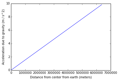
Acceleration vs Distance from center of the earth (uniform density)
It will be interesting to see in a graphical form, how the acceleration due to gravity varies by depth as one goes deeper into the earth. Lets calculate and plot this first. From our analytical work (ah=hRgah=hRg), its expected to be a linear relationship (so its not all that interesting after all).
def calc_acc_at_depth(d):
    """
    returns the acceleration at distance d
    from the center of the earth, assuming
    uniform density
    """
    if d > rad:
        return g
    if d < -rad:
        return -g
    vol_d = 4 * pi * pow(d, 3.0) / 3.0
    md = density * vol_d
    acc = G*md / pow(d, 2.0)
    return acc

acc_at_depth = []
for d in xrange(500, 1, -1):
    dd = d*rad / 500
    acc_at_depth.append((dd, calc_acc_at_depth(dd)))

xvals = [a for a,b in acc_at_depth]
yvals = [b for a,b in acc_at_depth]
plt.xlabel("Distance from center from earth (meters)")
plt.ylabel("Acceleration due to gravity (m / s^2)")
plt.plot(xvals, yvals)
The above graph is, as expected, a straight line, though there was hardly any doubt about that outcome.
Next, we will calculate and plot the travel time for 127 different tunnel lengths, uniformly distributed in their length, starting from 100 km and going up to 12700 km (almost equal to the diameter).
chord_lengths = [100000*n for n in range(1, 127)]

def get_acc(chlen, R, x):
    """
    return acceleration at distance x
    into a tunnel of length chlen
    """
    return (g/(2*R))*(chlen - 2*x)

def get_vt(s, v, a):
    """
    Given the current velocity, acceleration a distance 's',
    returns the velocity after train covers the distance 's'
    and the time take to cover the distance.
    """
    rv = rt = 0
    if a == 0:
        rv = v
        rt = s/v
        return (rv, rt)
    rt = (math.sqrt(v*v + 2*a*s) - v) / a
    rv = v + a*rt
    return (rv, rt)

def get_travel_time(chlen, nparts, acc_func):
    """
    returns the total travel time for traversing the
    tunnel, from beginning to end
    """
    dist = chlen/2.0
    curve_power = 2.0
    stfacs = [pow((float(x)/nparts), curve_power) for x in xrange(nparts+1)]
    steps = [dist*xx for xx in stfacs]
    total_time = 0
    cv = 0
    for st1, st2 in zip(steps, steps[1:]):
        dist = st2 - st1
        acc = acc_func(chlen, rad, st1)
        cv, time_part = get_vt(dist, cv, acc)
        total_time += time_part

    return 2*total_time

results = [(dist1, get_travel_time(dist1, 500, get_acc)) for dist1 in chord_lengths]

# plot of time vs chord length
yvals = [t/60.0 for d, t in results]
maxDiff = max(yvals) - min(yvals)

yvals = [float("%10.6f" % t) for t in yvals]
xvals = [d for d, t in results]
plt.xlabel("Length of tunnel (meters)")
plt.ylabel("Travel time (minutes)")
plt.plot(xvals, yvals)

print "Difference between max and min travel times : %s" % maxDiff
Output: Difference between max and min travel times : 2.69295696853e-12
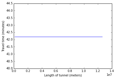
All right! This confirms our analytical solution. The travel time across chords of different length are indeed almost exactly the same. The differences in the max and min travel times is of the order of \(10^{−11}\), which is probably the best accuracy that we can get with double precision arithmetic on a computer.
This is all well and good for the simplified case of the earth having uniform density. But that is not true for the real earth. In fact, we expect the density near the core to be larger due to the pressure of all the mass that is pressing down upon it.
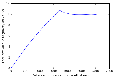
Acceleration in non-uniform density
This website (http://geophysics.ou.edu/solid_earth/prem.html) gives us a table of acceleration vs depth for the earth.
I copy pasted the table and cleaned up the data in a few lines of code below (python is awesome).
# depth vs acceleration table from
# http://geophysics.ou.edu/solid_earth/prem.html

g_at_depth = """0.0 11266.20    3667.80 13088.48    1425.3  176.1   0.4407  363.850 0.0000
200.0   11255.93    3663.42 13079.77    1423.1  175.5   0.4408  362.900 0.7311
400.0   11237.12    3650.27 13053.64    1416.4  173.9   0.4410  360.030 1.4604
600.0   11205.76    3628.35 13010.09    1405.3  171.3   0.4414  355.280 2.1862
800.0   11161.86    3597.67 12949.12    1389.8  167.6   0.4420  348.670 2.9068
1000.0  11105.42    3558.23 12870.73    1370.1  163.0   0.4428  340.240 3.6203
1200.0  11036.43    3510.02 12774.93    1346.2  157.4   0.4437  330.050 4.3251
1221.5  11028.27    3504.32 12763.60    1343.4  156.7   0.4438  328.850 4.4002
1400.0  10249.59    0.00    12069.24    1267.9  0.0 0.5000  318.750 4.9413
1600.0  10122.91    0.00    11946.82    1224.2  0.0 0.5000  306.150 5.5548
1800.0  9985.54 0.00    11809.00    1177.5  0.0 0.5000  292.220 6.1669
2000.0  9834.96 0.00    11654.78    1127.3  0.0 0.5000  277.040 6.7715
2200.0  9668.65 0.00    11483.11    1073.5  0.0 0.5000  260.680 7.3645
2400.0  9484.09 0.00    11292.98    1015.8  0.0 0.5000  243.250 7.9425
2600.0  9278.76 0.00    11083.35    954.2   0.0 0.5000  224.850 8.5023
2800.0  9050.15 0.00    10853.21    888.9   0.0 0.5000  205.600 9.0414
3000.0  8795.73 0.00    10601.52    820.2   0.0 0.5000  185.640 9.5570
3200.0  8512.98 0.00    10327.26    748.4   0.0 0.5000  165.120 10.0464
3400.0  8199.39 0.00    10029.40    674.3   0.0 0.5000  144.190 10.5065
3480.0  8064.82 0.00    9903.49 644.1   0.0 0.5000  135.750 10.6823
3600.0  13687.53    7265.75 5506.42 644.0   290.7   0.3038  128.710 10.5204
3630.0  13680.41    7265.97 5491.45 641.2   289.9   0.3035  126.970 10.4844
3800.0  13447.42    7188.92 5406.81 609.5   279.4   0.3012  117.350 10.3095
4000.0  13245.32    7099.74 5307.24 574.4   267.5   0.2984  106.390 10.1580
4200.0  13015.79    7010.53 5207.13 540.9   255.9   0.2957  95.760  10.0535
4400.0  12783.89    6919.57 5105.90 508.5   244.5   0.2928  85.430  9.9859
4600.0  12544.66    6825.12 5002.99 476.6   233.1   0.2898  75.360  9.9474
4800.0  12293.16    6725.48 4897.83 444.8   221.5   0.2864  65.520  9.9314
5000.0  12024.45    6618.91 4789.83 412.8   209.8   0.2826  55.900  9.9326
5200.0  11733.57    6563.70 4678.44 380.3   197.9   0.2783  46.490  9.9467
5400.0  11415.60    6378.13 4563.07 347.1   185.6   0.2731  37.290  9.9698
5600.0  11065.57    6240.46 4443.17 313.3   173.0   0.2668  28.290  9.9985
5701.0  10751.31    5945.08 4380.71 299.9   154.8   0.2798  23.830  10.0143
5771.0  10157.82    5516.01 3975.84 248.9   121.0   0.2909  21.040  10.0038
5701.0  10751.31    5945.08 4380.71 299.9   154.8   0.2798  23.830  10.0143
5771.0  10157.82    5516.01 3975.84 248.9   121.0   0.2909  21.040  10.0038
5871.0  9645.88 5224.28 3849.80 218.1   105.1   0.2924  17.130  9.9883
5971.0  9133.97 4932.59 3723.78 189.9   90.6    0.2942  13.350  9.9686
6061.0  8732.09 4706.90 3489.51 163.0   77.3    0.2952  10.200  9.9361
6151.0  8558.96 4643.91 3435.78 152.9   74.1    0.2914  7.110   9.9048
6221.0  8033.70 4443.61 3367.10 128.7   66.5    0.2796  4.780   9.8783
6291.0  8076.88 4469.53 3374.71 130.3   67.4    0.2793  2.450   9.8553
6346.6  8110.61 4490.94 3380.76 131.5   68.2    0.2789  0.604   9.8394
6356.0  6800.00 3900.00 2900.00 75.3    44.1    0.2549  0.337   9.8332
6368.0  5800.00 3200.00 2600.00 52.0    26.6    0.2812  0.300   9.8222
6371.0  1450.00 0.00    1020.00 2.1 0.0 0.5000  0.000   9.8156"""

g_at_depth = g_at_depth.strip().split("\n")
g_at_depth = [d.split("\t") for d in g_at_depth]
g_at_depth = [(float(d[0]), float(d[-1])) for d in g_at_depth]
g_at_depth = sorted(set(g_at_depth))

xvals = [d for d, g in g_at_depth]
yvals = [g for d, g in g_at_depth]
plt.xlabel("Distance from center from earth (kms)")
plt.ylabel("Acceleration due to gravity (m / s^2)")
plt.plot(xvals, yvals)
The PREM data only gives the acceleration at discrete intervals. We will write an interpolation method which will do a linear interpolation of the acceleration based on the PREM table.
After doing that, we can find the travel times for different chord lengths and plot it.
# find correct acceleration at varying depths
dtable = [d for d, g in g_at_depth]
gtable = [g for d, g in g_at_depth]

from bisect import bisect_left

def get_real_acc_at_depth(depth):
    """
    using linear interpolation of the PREM table, find the
    acceleration due to gravity at given depth and return it.
    """

    idx = bisect_left(dtable, depth)
    if idx == len(dtable) - 1:
        return gtable[-1]
    gl, gh = gtable[idx], gtable[idx+1]
    dl, dh = dtable[idx], dtable[idx+1]
    fac = (d - dl)/(dh - dl)
    rg = gl + fac*(gh - gl)
    return rg

def get_actual_acc(chlen, R, x):
    """
    return real world acceleration at distance x
    into a tunnel of length chlen
    """
    depth = math.sqrt(R*R + x*x - chlen*x)
    gd = get_real_acc_at_depth(depth/1000.0)
    return (gd/(2*depth))*(chlen - 2*x)


results = [(dist1, get_travel_time(dist1, 500, get_actual_acc)) for dist1 in chord_lengths]

# plot of time vs chord length
xvals = [d for d, t in results]
yvals = [t/60.0 for d, t in results]
plt.xlabel("Tunnel length (meters)")
plt.ylabel("Travel time (minutes)")
plt.plot(xvals, yvals)
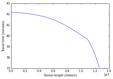
Whoa.... this is damn cool!
The graph above shows that we can travel to the opposite side of the earth in ~37 minutes, while it takes 42 minutes to travel to nearby places. This is the kind of result that makes one fall in love with physics and maths.
Maybe someday, we can find such a shortcut through space which allows us to jump to far away galaxies faster than we can travel in our own solar system.
If you look closely, you will also see that this is the essence of gravity assisted slingshot mechanisms that space rockets use to their advantage for gaining speed and venturing into outer space.
Comments